Algorithm Choice and Performance
Algorithms, and choosing the correct one, is a feature of all programming courses; Sorting algorithms are often used to demonstrate this: an approach that performs well on a small data set (for example, bubble sort) quickly becomes unusable at scale, requiring fundamentally different strategies such as heap sort.
This article is based on a real situation that occurred with the Tekton Lint tool. The concept of this tool is to read a Tekton yaml file and process it to find semantic errors such as parameter defined but never used, preferred format of task names.
The discussion below is presented in a (roughly) linear manner to demonstrate the thought processes and answer the question like these: How was the problem inspected? What a solution to the problem could be? And finally, how the implementation and testing took place.
Tl;Dr; Performance was improved by several orders of magnitude.
Problem report
The linting of a large file (auto-generated) was taking a “long time”; initial investigations by the reporter determined that a similar number of tasks when separated out didn’t have the same behaviour. On the definition of a long time, for a CLI tool this is subject to the human perception of time. In this case a tool that would usually be seen to run in a few seconds, was taking minutes.
IO is the slowest part of a system, would not more files have been slower due to the file IO?
The reporter had also determined that the file in question had 3300+ warnings reported, and with the majority being one specific rule. All the warnings were valid, so this wasn’t a false positive result.
Was it something about this rule that was amiss? There is a lot of iteration in the rules to check values.
The report concluded with the context that this was run in Kubernetes, and was hitting pod CPU limits; this is useful information as it dismisses any initial thoughts about IO and this is looking to a CPU based problem. Being CPU bound is suggesting an algorithm related issue. The reporter was kind enough to send the original file, **88864 lines 2.9Mib **. This is always a great help as a local recreation of the problem can happen.
On reproducing the problem clearly showed the issue; the time command shows the time spent.
$ time node dist/lint.js large_file.yaml
217.40s user 9.97s system 100% cpu 3:45.63 total
A run time of 3 minutes 45 seconds is a long time for a CLI together with reports of the Kubernetes Pod hitting resource limits, this is certainly a problem that needs addressing. Whilst a 3 MiB YAML file is large, and could be questioned in this case it came via automation tooling so was not unreasonable.
Analysis starts
With any performance problem if you are able to get a performance profile it will allow the analysis to be much more effective. In this case with a single Node.js process obtaining a profile of the code execution is trivial. Sometimes it is not so easy, especially if the performance issue is between distributed systems or processes. However, profiling provides real hard data, so it is worth putting in effort to get this information.
Node.js has built in profiling tools; running the code with the --prof options take measurements, and produce a couple of reports
$ node dist/lint.js large_file.yaml

.rw-r--r-- 5.2M matthew  4 Apr 09:23 -N isolate-0x5e804a0-538778-v8.log
.rw-r--r-- 3.5M matthew  4 Apr 09:23 -N isolate-0x7f5a18001000-538778-v8.log
These need to be processed to produce a report, for example
node --prof-process isolate-0x5ee14a0-525429-v8.log > op2.log
Node.js works on a event based system, and therefore counts in ticks; the JavaScript reports (there are also reports for C/C++) clearly shows the top three ‘culprits’ _getLocation/_getLine/_getCol
 [JavaScript]:
   ticks  total  nonlib   name
  46173   26.2%   27.7%  JS: *_getLocation file:///home/matthew/github.com/mbwhite/tekton-lint/dist/reporter.js:79:17
  15644    8.9%    9.4%  JS: *_getLine file:///home/matthew/github.com/mbwhite/tekton-lint/dist/reporter.js:62:13
  13976    7.9%    8.4%  JS: *_getCol file:///home/matthew/github.com/mbwhite/tekton-lint/dist/reporter.js:70:12
     47    0.0%    0.0%  JS: *next /home/matthew/github.com/mbwhite/tekton-lint/node_modules/yaml/dist/parse/parser.js:167:10
     44    0.0%    0.0%  JS: *parseDocument /home/matthew/github.com/mbwhite/tekton-lint/node_modules/yaml/dist/parse/lexer.js:316:19
     33    0.0%    0.0%  JS: *resolveBlockMap /home/matthew/github.com/mbwhite/tekton-lint/node_modules/yaml/dist/compose/resolve-block-map.js:11:25
     32    0.0%    0.0%  JS: *walk file:///home/matthew/github.com/mbwhite/tekton-lint/dist/walk.js:1:21
     31    0.0%    0.0%  JS: *parsePlainScalar /home/matthew/github.com/mbwhite/tekton-lint/node_modules/yaml/dist/parse/lexer.js:556:22
     22    0.0%    0.0%  JS: *step /home/matthew/github.com/mbwhite/tekton-lint/node_modules/yaml/dist/parse/parser.js:231:10
     20    0.0%    0.0%  JS: *blockMap /home/matthew/github.com/mbwhite/tekton-lint/node_modules/yaml/dist/parse/parser.js:475:14
     19    0.0%    0.0%  JS: *lex /home/matthew/github.com/mbwhite/tekton-lint/node_modules/yaml/dist/parse/lexer.js:152:9
     19    0.0%    0.0%  JS: *findScalarTagByTest /home/matthew/github.com/mbwhite/tekton-lint/node_modules/yaml/dist/compose/compose-scalar.js:67:29
     19    0.0%    0.0%  JS: *composeScalar /home/matthew/github.com/mbwhite/tekton-lint/node_modules/yaml/dist/compose/compose-scalar.js:8:23
     17    0.0%    0.0%  JS: *resolveProps /home/matthew/github.com/mbwhite/tekton-lint/node_modules/yaml/dist/compose/resolve-props.js:3:22
     17    0.0%    0.0%  JS: *parseNext /home/matthew/github.com/mbwhite/tekton-lint/node_modules/yaml/dist/parse/lexer.js:223:15
     15    0.0%    0.0%  JS: *pushIndicators /home/matthew/github.com/mbwhite/tekton-lint/node_modules/yaml/dist/parse/lexer.js:619:20
     13    0.0%    0.0%  JS: *pop /home/matthew/github.com/mbwhite/tekton-lint/node_modules/yaml/dist/parse/parser.js:270:9
     12    0.0%    0.0%  JS: *pushSpaces /home/matthew/github.com/mbwhite/tekton-lint/node_modules/yaml/dist/parse/lexer.js:681:16
     12    0.0%    0.0%  JS: *parseLineStart /home/matthew/github.com/mbwhite/tekton-lint/node_modules/yaml/dist/parse/lexer.js:280:20
     12    0.0%    0.0%  JS: *parse /home/matthew/github.com/mbwhite/tekton-lint/node_modules/yaml/dist/parse/parser.js:156:11
      8    0.0%    0.0%  RegExp: \s+$
      7    0.0%    0.0%  JS: *resolveBlockSeq /home/matthew/github.com/mbwhite/tekton-lint/node_modules/yaml/dist/compose/resolve-block-seq.js:7:25
Based on the knowledge of the code, these are not specifically then the rule itself, but the reporting of the rule; this gives an indication though of a real issue and where to start.
Code Inspection
The code presented here is almost the same as the original code; the original code is Apache-2.0 Open source and is available. The replication here was used to develop the end solution, and when this was fitted into the real code worked (almost - more later) as expected.
To perform the checks, the tool has read the text file into memory; this has been parsed and a set of rules are then run over the parsed syntax. When a problem is reported the character offset from the start of the file is known. Based on this offset we need to know the line number and column number of that character offset. This is so it can be reported to the user, who can then easily find it.
Given an offset of a character into a source code (text) file, calculate the line number and column of that offset
Code Analysis
The entry point is the first function _getLocation
    _getLocation(s: string, n: number): Result {
        if (!this.preCreateArray) this.dataarray = Array.from(s);
        const chars = this.dataarray;
        const l = this._getLine(chars, n);
        const c = this._getCol(chars, n);

        return new Result(l, c);
    }
In the case of finding several errors in the same file, there will be repeated calls to _getLocation(). So for the original problem this means that this function is called >3000 times.
Each time this is called, it is passed the full raw value of the file as a single string, along with a number being the character offset into the string. It returns the line and column of this character using the _getLine/_getCol functions. Note the first line in the code is the this.dataarray = Array.from(s); this converts from a string into an array of characters.
This array conversion is happening every time, but the data isn’t changing; an optimization here is to cache the result of this conversion. To demonstrate this change, we can run 3000 iterations on varying size files and track the time. This graph is showing the average time per iteration for each input data size.
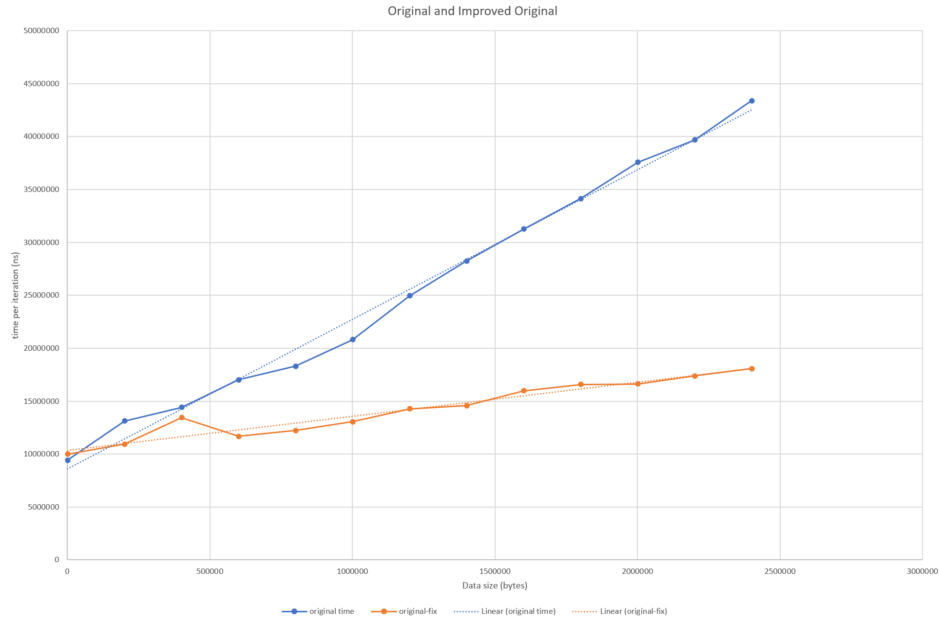
It has certainly helped with the gradient; the changing size of the input file has less effect, but the overall order of magnitude is still the same. In reality the user would be still be waiting minutes though.
Looking back at the profile shows that the other two functions also have a lot of time spent in them. So by reviewing just the profiling data, we can that removing this array conversion will help though it’s not the whole story.
Looking at the next two functions, for the line and column number; these are simple iterative functions.
    _getLine(chars: string[], n: number): number {
        let l = 1;
        for (let i = 0; i < n; i++) {
            if (chars[i] === '\n') l++;
        }

        return l;
    }

    _getCol(chars: string[], n: number): number {
        let c = 1;
        for (let i = 0; i < n; i++) {
            if (chars[i] === '\n') c = 0;
            c++;
        }
        return c;
    }
Both work similarly, they take the array of characters and an offset. They iterate over the arrays up to the offset. In the case the _getLine this counts the number of \n or newline characters it’s seen. _getCol counts characters, but resets the count at newlines.
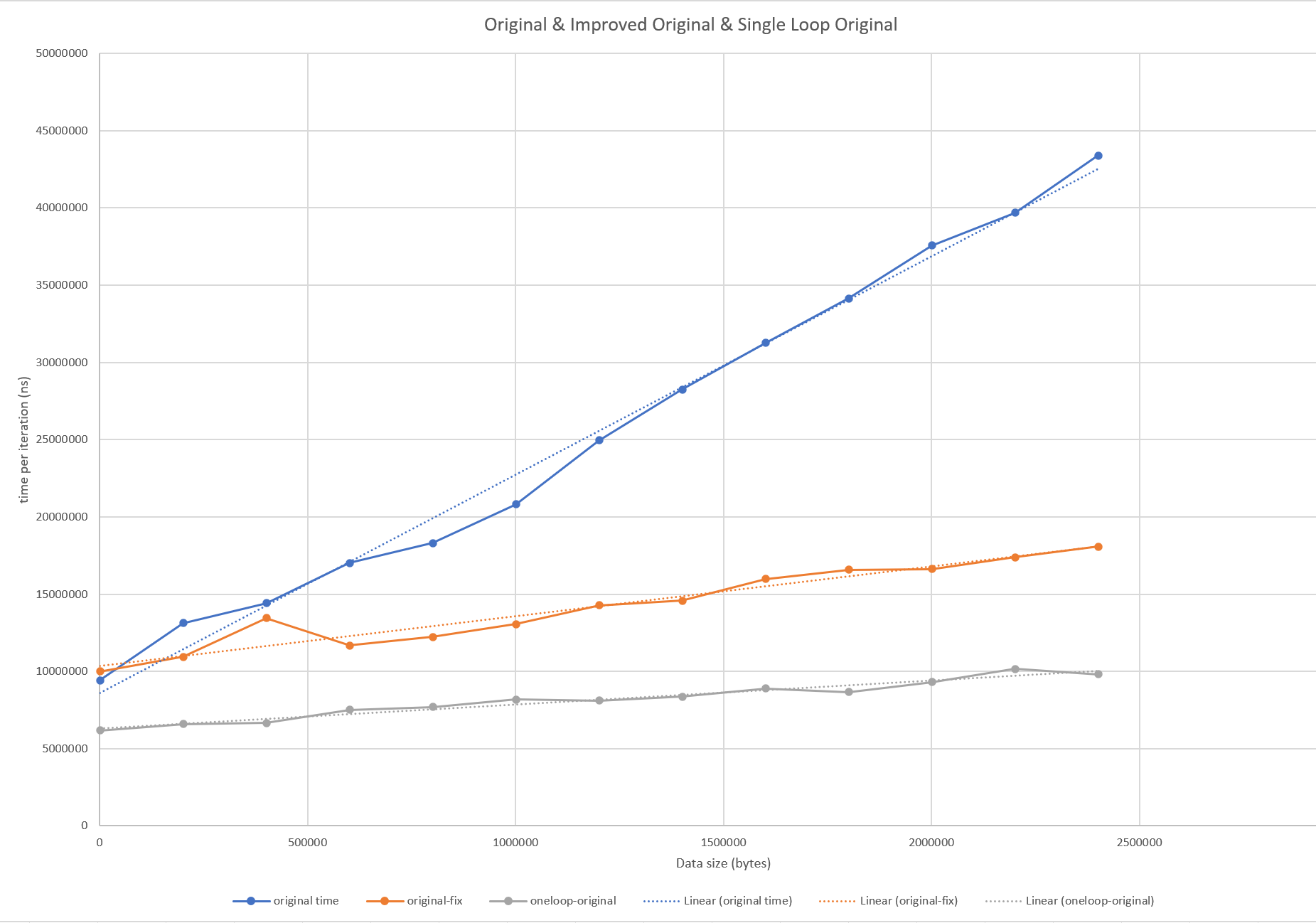
The two loops are very similar, and they could be combined into a single iterative loop. This would also help overall time - as seen in the graph below.
Whilst we’ve been able to reduce the impact of the increasing file size, the function is still expensive given a large data file. If the offset is at the start of the file, it’s not so bad, but at worst case the file has to searched from the start. Similarly, if only one offset needs to be calculated this is not so bad. If the graphs are recreated with say only 10 iterations, the performance of the original can be seen to improve especially if the randomly selected offsets tend to lower values.
The gradient of the line is slightly flatter, but the number of comparisons though needed to find the line and col from offset is still in linear relationship with the size of the data.
Tree Data Structures
When using searches, rather than a linear search a data-structure that is useful is a ‘tree’ - particularly the Binary Search Tree
We can use a variation of such a tree here; the downside is that the code above is simple, with a few modifications we’ve improved the performance. But we’ve the same order of magnitude. To get better results we need to pick different search algorithms, but this comes at the expense of more code complexity.
To summarize, the tree has a root (computer science trees have their roots at the top not bottom!) the node can store whatever data it likes, but there must be some ‘key’ which can be compared to know whether the next node should go the left or right.
Here we’re going to use the ‘key’ being the range of characters for a line. The table shows an how this can be represented. The X in the table represent the characters in the source code file with the columns and lines marked. At the end of each line is the character offsets of the start and end characters of each line. (a blank means no character at all)
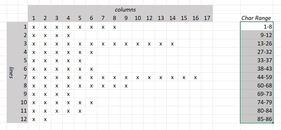
So the first line has a character offset range 1-8, second line, 9-12, third 13-26. Note that the newline characters are included in the count of the characters. The code does need to be mindful of the 0 based nature of the arrays, but the counting of rows/columns is 1 based, as is the offset
For the character offset ranges, we can create a tree. Where each node in the tree has a value that is one of these ranges.
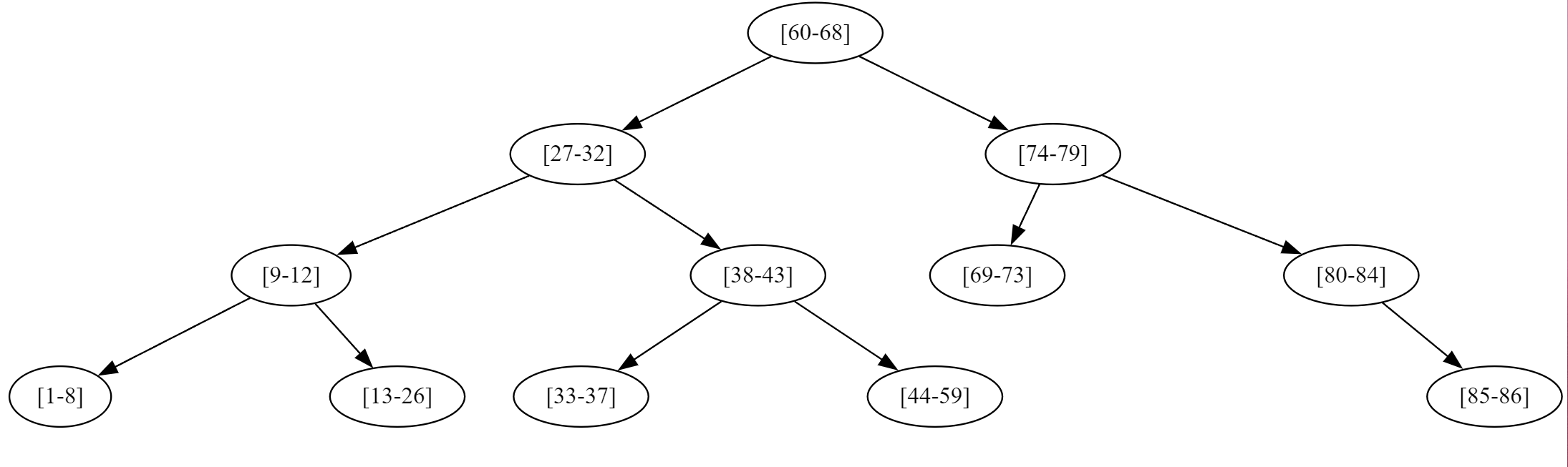
The root is the node representing the range [60-68] To it’s left, is the [27-32] range, and right [74-79] To add nodes to a tree, a comparator function is needed to know if the new node should go to the left (and be ‘smaller’) or the right (and be ‘larger’).
Here the comparator function needs to ensure that [27-32] is less than [60-98] the root but [74-80] is greater than the root. When it comes to searching though we don’t have a range, but a single value, eg offset 19; similarly a carefully created comparator function will let us return the second line’s node as the matching one. The node that has the range that 19 will fall in is the [9-12] node. Again the search will proceed down the tree from the root, directing the search initially to the left to [27-32] and then left to [9-12], then to the right to [13-26], 19 is in this range, so the search has concluded.
The values held in the nodes or the links is entirely open, and in this case each node can store both the range and also a value that represents the line number.
This can return the line number of 3, the column offset can be calculated based starting range (13) 19-13-1 (not forgetting the -1 - offset by 1 errors are very common!)
The central compare function
    public compare(other: IndexRange): number {
        if (this.isQuery()) {
            if (this.start >= other.start && this.start <= other.end) {
                return 0;
            }
        }

        if (other.isQuery()) {
            if (other.start >= this.start && other.start <= this.end) {
                return 0;
            }
        }

        if (this.start > other.end) {
            // goes to the right as larger
            return 1;
        } else if (this.end <= other.start) {
            return -1;
        }

        // which should in theory never happen
        return 0;
    }
The first two if statements are there to handle the case where we are searching for node, i.e. we just have the offset. The isQuery function determines this, and if the searched for offset is in within the range, then 0 is returned meaning a match.
The second two if statements determine if the range (or search) will be located either to the left or right (i.e. less or more) of this node.
Implementation of the tree data-structure and insertion of nodes are standard well documented knowledge, and once a specific comparator function is supplied, the implementation is ignorant of the types of data.
There is only critical aspect though to the use of tree data-structures, in that for efficiency they must be ‘balanced’ or at least approach balance; for any given node, the size of the left subtree and right subtree must have similar depths. If for example a set of integers is added starting wit the smallest, 1,2,3,4,5…. then each new node created will always be to the right of the first node; this is the worst case scenario and will create unbalanced tree that is effectively a list. In the tree diagram above this is balanced well, visually it’s quite easy to see that it has a large amount of symmetry.
As the nodes we are creating come from the lines of the file and the character offsets, starting at the top of the file and running through it line by line will create a completely unbalanced tree.
A simple, but effective solution is to randomize the inputs to the tree. The chart below (note it has a log vertical scale for the time per iteration) shows how the updated data-structure provides significant improvements if and only if the tree is in any way balanced.
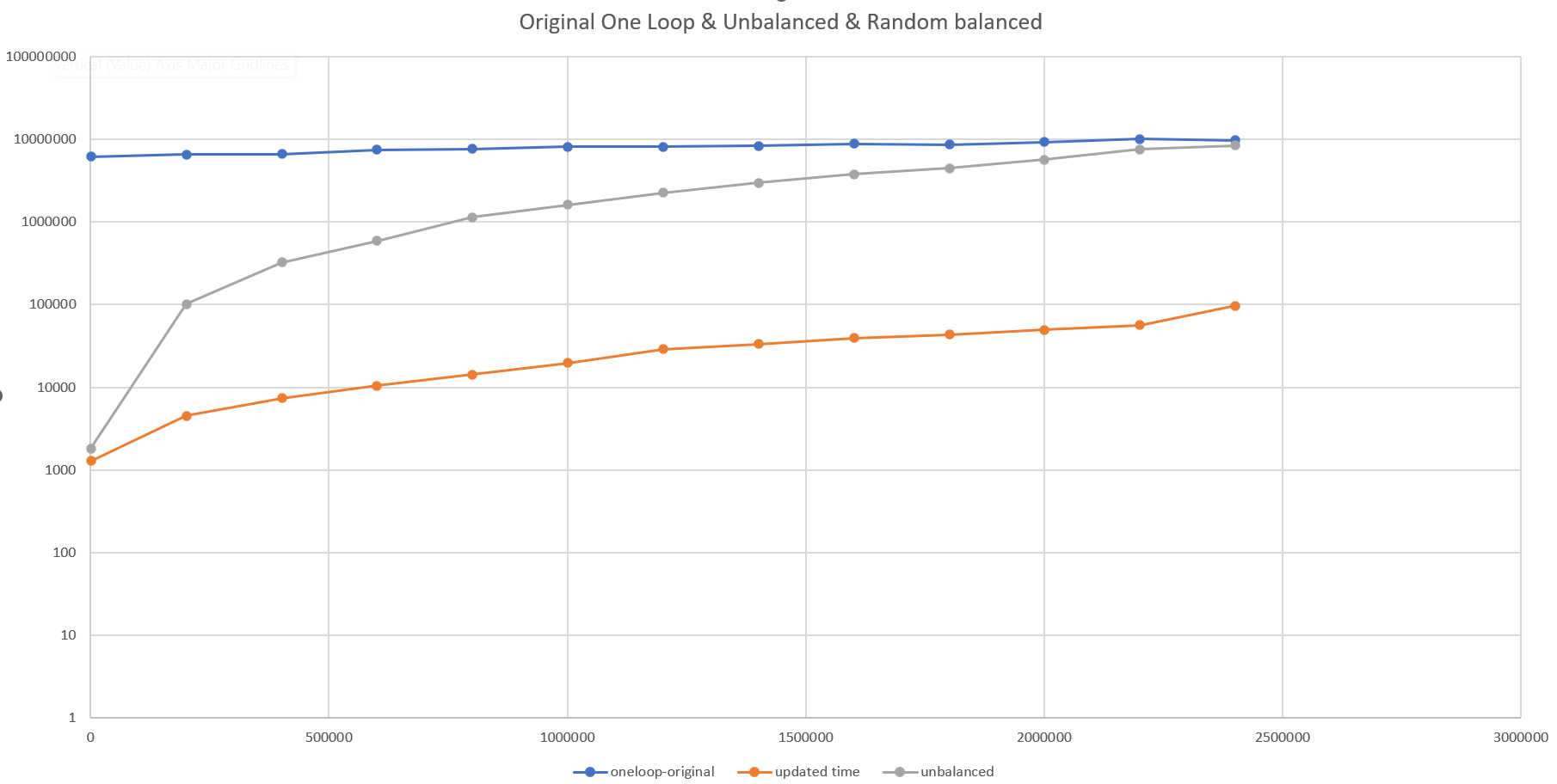
The unbalanced tree results in awful performance, but when the input data is randomized as in this case, we get much improved results.
Critically here though the reduction in order of magnitude of the problem, but at least 3 orders of magnitude. In practice this takes the execution of the code from minutes (3m:45s) for the large file to seconds (0m:04s).
For the situation here the data is known up front, and added to the tree, for searching. Nothing will be added later or removed. The random insertion of data is a valid solution; although possibly lacks elegance. If data was being continually added and/or removed this would be an invalid solution. Without rebalancing, the tree would get worse over time.
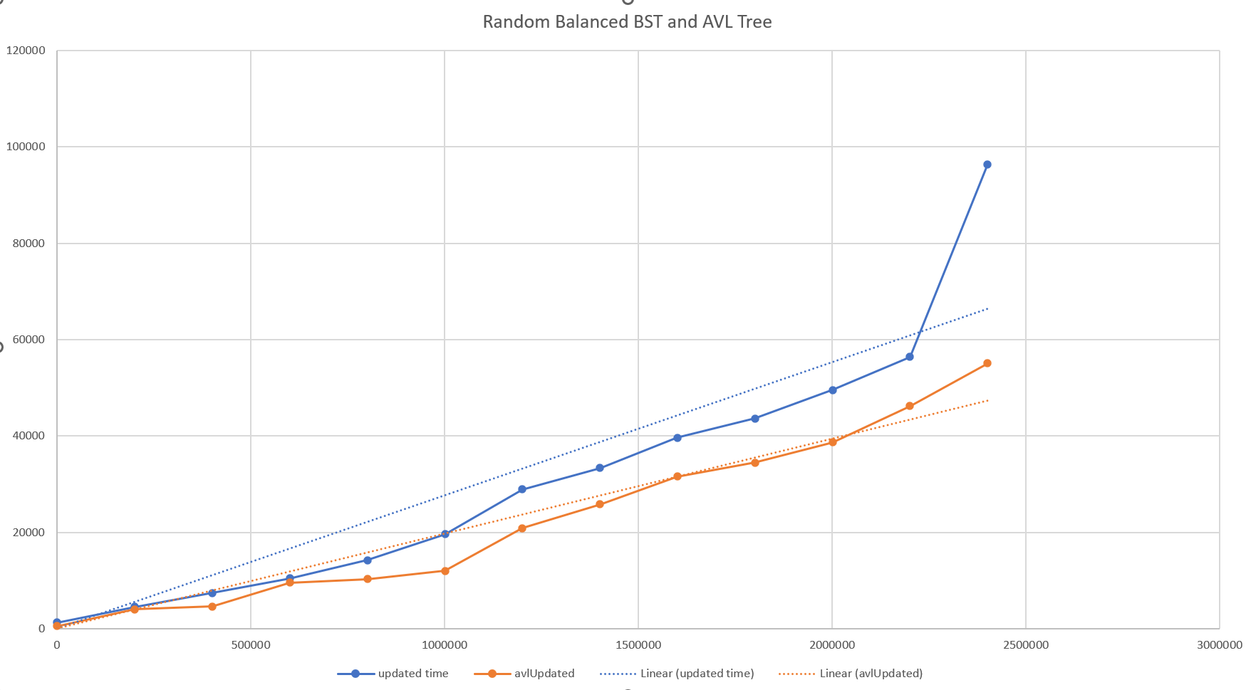
There is one final improvement that was investigated; this is to produce a variant of the tree that is self-balancing on insertion - specifically the AVL tree. Again the complexity here increases; each insertion records the depth of the nodes, and if any node is showing an imbalance between left and right a set of ‘rotations’ is performed to correct the imbalance.
This doesn’t produce perfectly balanced trees, but the results are very close, and the advantage is that the tree remain in this state during all insertions and deletions. And it does produce a more balanced tree than a randomized one.
As the tree is more balanced the performance is improved as seen below.
Final Implementation Notes
As alluded to above, when this updated algorithm was implemented in the actual code it almost worked.
Out-of-memory
This occurred on the first test, run Node.js processed failed with an out of memory error. By introducing a new data-structure, more memory was being consumed, but the structure itself is small. What is relevant is that the data-structure was part of the bigger picture of the application. Within that application there is another tree representing the Tekton components of the parsed YAML file. Each of these nodes had a reference to the complete data of the file - and when the new structure had been added each of these nodes had been given its own copy.
This was redundant, so a simple caching system was implemented giving only 1 tree per raw data file.
Functional Errors
Functional tests in the application also picked up a couple of errors; the behaviour of the new data-structure was working well, but in some cases the line/column reported where slightly different from previously.
Edge cases such as this are an always present concern for algorithms that seek to generalize functionality. In this case the edge cases where were the reported ranges occurred at the end of files, and if the files had blank lines at the end or not.
It also demonstrates the ‘off-by-1’ error that is often seen and can be very hard to finally ‘pin down’. The best advice here is to proceed slowly and carefully. Carefully checking the handling the 0 and 1 based indexing was the solution here.
Final Profiling
A final performance profile was taken of the code; the result here showed none of the previously seen functions. Along with the empirical boost in speed, this was good evidence a major issue had been solved.
What the profile did show was the functions that now consumed the bulk of the time, where the ones that were related to initially parsing and locating all the YAML files. There was no reason to investigate more here.